Modelování vnitřní teploty pomocí programů TRNSYS a MATLAB/SIMULINK
Cílem této práce bylo navrhnout počítačový model pro simulaci vnitřního prostředí v budovách během letního období. Model byl vytvořen v programu TRNSYS a MATLAB/SIMULINK. Simulace byly provedeny pro jednu z přednáškových místností Fakulty strojního inženýrství Vysokého učení technického v Brně. Výpočet dopadajícího slunečního záření na vnější povrchy budovy byl proveden v programu TRNSYS, na základě skutečných dat z meteorologické stanice v Brně (TUBO). V programu MATLAB/SIMULINK pak byl proveden vlastní výpočet teploty vzduchu v místnosti a model byl validován pomocí dat z monitorovacího systému instalovaného v budově fakulty. Výsledky simulací dobře odpovídaly naměřeným hodnotám.
1. Introduction
Some methods are used to simulate the energy in buildings for predicting energy consumption and to determine the parameters of the indoor climate. Where, the results are used then to design building as required, so that to be able to meet the different requirements for energy consumption and indoor climate. The main principle of building energy simulation is to determine all the energy flows [1]. Heat losses are through the building envelope (windows, walls ceiling and the floor), as well as through the ventilation system and infiltration. While thermal gains basically represent the solar heat gain through windows, internal heat from people, lighting and equipment. These variables are continuously changing. Therefore air conditioning system must take these facts into account in order to maintain an acceptable temperature indoor with reducing energy consumption to a minimum.
In a mathematical model representing indoor environment, all what may affect the energy balance must be included in the model. It means that sub-models for walls, windows, and all other components inside the building must be modelled.
The MATLAB environment has advanced capabilities to simulate indoor thermal processes. A whole building model has already been developed in MATLAB. This model, called HAMBase (Heat, Air and Moisture model for Building and Systems Evaluation) [2], and is one of the oldest simulation tools based on MATLAB environment in order to model the heat and humidity in the building. Where, with the model of indoor temperature, indoor humidity and energy required for heating and cooling can be simulated for a multi-zone building. This model has continuously been improved and implemented in MATLAB. Important features for this work are: multi-zone modelling, solar and shadow calculations and multi climate conditions.
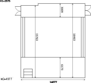
Fig. 1 Dimensions of the building
The classroom being modelled in this work is separated from the outdoors by an external wall and a window, and from adjoining rooms at the sides by internal partitions, and at above and below by a ceiling and a floor slab. Figure 1 shows a diagram of the building, where, the main dimensions in mm are clarified.
The volume of indoor space in this work is 910 m3. There are two external walls with the same dimensions. One of them in north-northwest orientation, while the other in south-southeast orientation. Each wall is covered partially with a wood layer. Area of wood is 28.63 m2, while area of concrete is 14.65 m2. There is a window in each wall included inside steel frame. Area of glass is 9.64 m2, while area of frame is 4.35 m2. There is another external wall with orientation east-northeast. It is covered partially with a wood layer too, with the same layers. Area of wood is 36.65 m2, while area of concrete is 33.40 m2.
With regard to roof, there is an air gap with thickness 300 mm assumed that has the same indoor temperature. Then, there is concrete layer. Above roof, there is a room containing equipment for HVAC system. Its temperature changes between the indoor and outdoor temperatures, and it has been obtained by direct measurement. Area of the roof is 231.75 m2.
Further data are in Table 1.
| Material | Thickness [mm] | Thermal conductivity [W/m.K] | Specific heat capacity [J/kg.K] | Density [kg/m3] |
|---|---|---|---|---|
| Wood | 5 | 0.17 | 2000 | 700 |
| Concrete | 25 | 1.7 | 920 | 2300 |
| Brick | 450 | 0.8 | 800 | 1700 |
| Steel | 30 | 16 | 490 | 7820 |
There is an inner wall connected with conditioned indoor space, while under the floor there is another classrooms conditioned too. It is assumed that the heat exchanges between the inner wall and the floor on the hand, with the classroom on the other hand, are neglected.
The heat transfer processes that would take place in a building include:
(a) Conduction heat transfer through the building fabric elements, including the external walls, roof, ceiling and floor slabs and internal partitions.
(b) Solar radiation transmission and conduction through window glazing.
Outdoor climatic data have been obtained from meteorological station located in Brno city in Czech Republic, and is identified by four-character code “TUBO” [3].
The modelling has been applied for a hot summer day and there is no occupancy. HVAC system was turned off. The modelling results have been compared with the results of a monitoring system installed inside to validate the modelling.
2. TRNSYS model
External surfaces of buildings receiving solar radiation are generally tilted, except for the flat roof, which is a horizontal surface. Consequently, it is required to estimate radiation on such surfaces from the data measured on a horizontal surface. The tilted surfaces receive three types of solar radiation [4], are beam radiation directly from the sun, diffuse radiation coming from the sky dome, and reflected radiation due to neighbouring buildings and objects. The estimation of the last component is very complicated. However, its contribution is much less compared to the first two sources. Hence, reflected radiation due to neighbouring buildings and objects has been neglected in the model.
As for the available values of the intensity of solar radiation obtained from TUBO station, these values represent the intensity of radiation incident on the horizontal surface, so it is necessary to find some way from which to take advantage of these data to calculate the intensity of solar radiation incident on the external walls in the building, which are vertical surfaces with different orientations. The solution has been proposed by creating a model by using TRNSYS software which can provide a suitable simulation environment to model climate change [5]. The intensity of solar radiation incident on each external wall of the building can be calculated by using the values of temperature, relative humidity and the intensity of solar radiation on horizontal surfaces after knowing values describing the geographical location of the building, and azimuth angles of the walls.
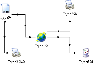
Fig. 2 TRNSYS model
The designed model is shown in Figure 2. Where the Solar Radiation Processor of this model includes: Total solar radiation on horizontal surface, Temperature and Relative Humidity.
This instance of Type16 takes hourly integrated values of total horizontal solar radiation and computes the diffuse fraction using an algorithm that estimates cloudiness based on dry bulb and dew point temperature. It can use various algorithms to compute radiation on tilted surfaces such as Hay and Davies, Perez, Reindl, etc. Data can be entered in solar or in local time.
The basic parameters in this model are as follows:
- Surface Tracking Mode: tracking mode is 1, because it is fixed surface.
- Starting day: The day of the year corresponding to the simulation start time, is 220 here.
- Latitude: The latitude of the location being investigated. Latitude for the building area is 49 degrees north.
- Solar constant: is 4871.0 kJ/hr.m2.
- Shift in solar time: Since many of the calculations made in transforming insolation on a horizontal surface depend on the time of day, it is important that the correct solar time be used. This parameter is used to account for the differences between solar time and local time. The equation for the shift parameter is: SHIFT = Lst − Lloc. Where: Lst is the standard meridian for the local time zone. Lloc is the longitude of the location. Longitude angles are positive towards West, negative towards East. The longitude here is 16.
The UTC is time used in TUBO data, is basically GMT (0 meridian). The shift is therefore 0 −(−16) = 16.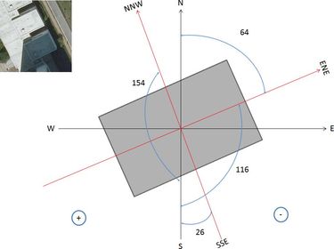
Fig. 3 Azimuth of surfaces - Slope of surface: The slope of the surface or tracking axis. 0 = Horizontal, while 90 = Vertical facing toward azimuth. For all walls, slope is 90.
- Azimuth of surface: The solar azimuth angle is the angle between the local meridian and the projection of the line of sight of the sun onto the horizontal plane. Building has three external walls with the following (approximate) orientations: north-northwest (NNW), south-southeast (SSE) and east-northeast (ENE).
Figure 3 illustrates these angles and method of calculation.
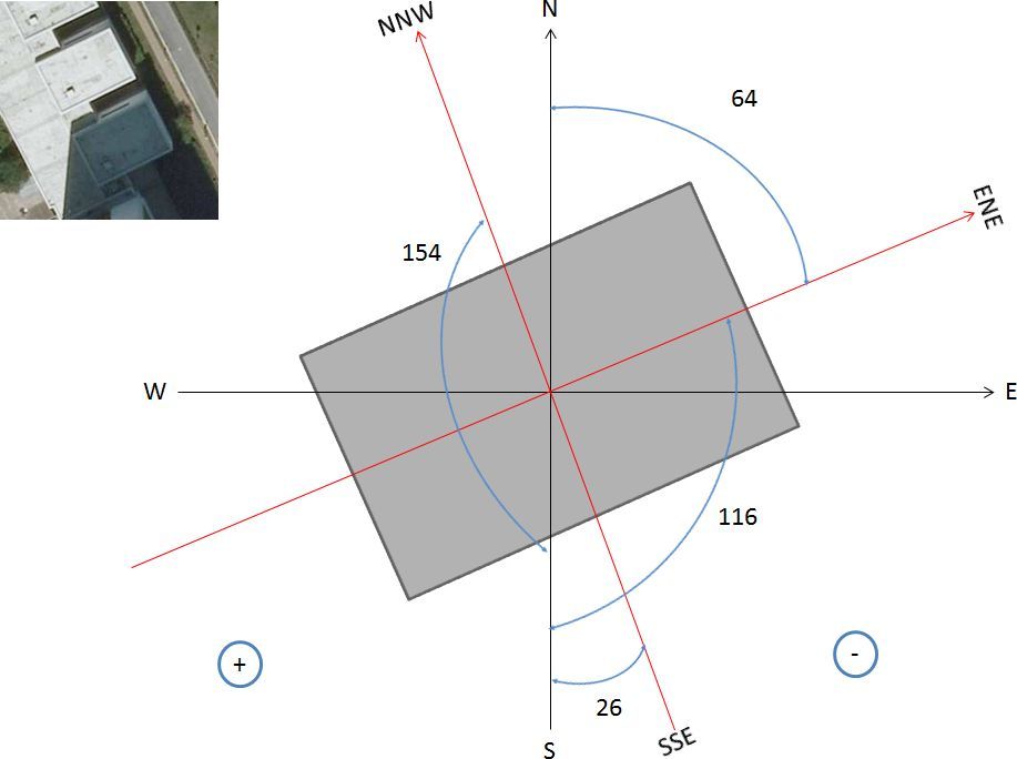
The results are as shown in Table 2.
| Wall | NNW | SSE | ENE |
| Azimuth | 154 | −26 | −116 |
Through this model, the values of solar radiation incident on each wall in the building can be calculated, then these data can be converted into MAT files, so that can be used in the model which has been designed by using MATLAB/SIMULINK.
3. SIMULINK model
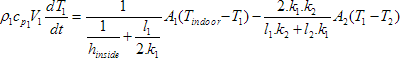
Energy balance in the classroom can be expressed by the following equation [6]:Where
- ρair
- is density of air [kg/m3]
- cp air
- – specific heat capacity of air [J/(kg.K)]
- Vindoor
- – indoor space volume [m3]
- Cinternal
- – lumped thermal capacity of the building, which is the sum of the internal capacities of all internal layers [J/K], where, building does not respond instantaneously to the changing heat, whether from outdoor or indoor sources. The rate by which the building will be conditioned depends largely on its thermal mass. The degree to which comfort conditions can be achieved depends not only on indoor temperature, but also on the temperature of the indoor surfaces. The effect of thermal mass may have a great effect on the energy performance of the building. The higher the heat capacity indoor the greater the building time constant. Consequently, the thermal response of the building to temperature fluctuations will take longer.
- Tindoor
- – indoor temperature [K]
- Qenvelopes
- – heat exchange through building envelopes [W]
- Qwindows
- – heat exchange through windows [W]

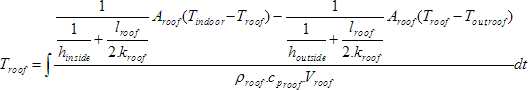
Fig. 4 Layers of the external wall
It is assumed that indoor air temperature and the temperature of all internal layers are the same.
According to Figure 4, heat transfer through the building envelopes can be expressed by the following equation [7]:

(2) [W]
Where
- hinside
- is heat transfer coefficient inside [W/m2.K]
- l1
- – thickness of wood layer (first layer inside) [m]
- k1
- – thermal conductivity of wood layer (first layer inside) [W/m.K]
- A1
- – area of wood layer (first layer inside) [m2]
- T1
- – temperature of wood layer (first layer inside) [K]
- lframe
- – thickness of windows frame [m]
- kframe
- – thermal conductivity of windows frame [W/m.K]
- Aframe
- – area of windows frame [m2]
- Tframe
- – temperature of windows frame [K]
- lroof
- – thickness of concrete layer of roof [m]
- kroof
- – thermal conductivity of concrete layer of roof [W/m.K]
- Aroof
- – area of concrete layer of roof [m2]
- Troof
- – temperature of concrete layer of roof [K]
Energy balance equation for wood layer (first layer inside) can be expressed by the following equation [7]:
 (3)
[W]
(3)
[W]
Where
- ρ1
- is density of wood layer (first layer inside) [kg/m3]
- cp1
- – specific heat capacity of wood layer (first layer inside) [J/kg.K]
- V1
- – volume of wood layer (first layer inside) [m3]
- k2
- – thermal conductivity of first concrete layer (second layer inside) [W/m.K]
- l2
- – thickness of first concrete layer (second layer inside) [m]
- A2
- – area of first concrete layer (second layer inside) [m2]
- T2
- – temperature of first concrete layer (second layer inside) [K]
By rearranging equation (3), T1 can be calculated as follows:
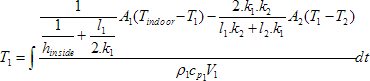 (4)
[K]
(4)
[K]
According to equation (4), temperature of next layer must be calculated. Hence, energy balance equation for first concrete layer (second layer inside) can be expressed by the following equation [7]:
Where
- ρ2
- is density of first concrete layer (second layer inside) [kg/m3]
- cp2
- – specific heat capacity of first concrete layer (second layer inside) [J/kg.K]
- V2
- – volume of first concrete layer (second layer inside) [m3]
- k3
- – thermal conductivity of brick layer (third layer inside) [W/m.K]
- l3
- – thickness of brick layer (third layer inside) [m]
- A3
- – area of brick layer (third layer inside) [m2]
- T3
- – temperature of brick layer (third layer inside) [K]
By rearranging equation (5), T2 can be calculated as follows:
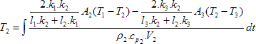 (6)
[K]
(6)
[K]
According to equation (6), temperature of next layer must be also calculated. Hence, energy balance equation for brick layer (third layer inside) can be expressed by the following equation [7]:
Where
- ρ3
- is density of brick layer (third layer inside) [kg/m3]
- cp3
- – specific heat capacity of brick layer (third layer inside) [J/kg.K]
- V3
- – volume of brick layer (third layer inside) [m3]
- k4
- – thermal conductivity of second concrete layer (fourth layer) [W/m.K]
- l4
- – thickness of second concrete layer (fourth layer) [m]
- A4
- – area of second concrete layer (fourth layer) [m2]
- T4
- – temperature of second concrete layer (fourth layer) [K]
By rearranging equation (7), T3 can be calculated as follows:
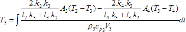 (8)
[K]
(8)
[K]
To calculate the effect of solar radiation, sol-air temperature is used, which is an equivalent outdoor temperature combines the effects of convection and radiation. Solar radiation on walls warms the surfaces and affects the rate of conduction heat transfer through the wall. It is calculated using the relation [8]:
Where
- Toutdoor
- is outdoor air temperature [K]
- I
- – the total solar heat flux on the wall [W/m2]
- α
- – absorptance of surface for solar radiation
By the same way, according to equation (8), temperature of next layer must be also calculated. Hence, energy balance equation of second concrete layer (fourth layer) can be expressed by the following equation [7]:
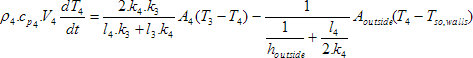 (10)
[W]
(10)
[W]
Where
- ρ4
- is density of second concrete layer (fourth layer) [kg/m3]
- cp4
- – specific heat capacity of second concrete layer (fourth layer) [J/kg.K]
- V4
- – volume of second concrete layer (fourth layer) [m3]
- Aoutside
- – area of outside surface [m2]
- Tso,walls
- – sol-air temperature for external walls [K]
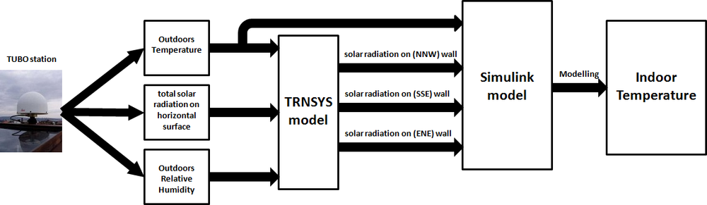
Fig. 5 Modelling the intensity of solar radiation on each wall
Considering that there are three external walls in different orientations, there are three different values of sol-air temperatures, depending on the intensity of solar radiation incident on each wall. Where, values of intensity of solar radiation incident on each wall have been calculated by using TRNSYS model as shown in Figure 5.
By rearranging equation (10), T4 can be calculated as follows:
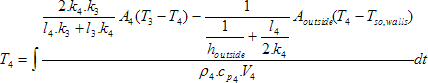 (11)
[K]
(11)
[K]
After calculating temperatures of all layers, T1 can be calculated, and then the first quantity of the right side of equation (2) can be calculated.
Energy balance equation of frame can be expressed by the following equation [7]:
 (12)
[W]
(12)
[W]
Where
- ρframe
- is density of frame [kg/m3]
- cp frame
- – specific heat capacity of frame [J/kg.K]
- Vframe
- – volume of frame [m3]
- Tso frame
- – sol-air temperature for frame [K]
By rearranging equation (12), Tframe can be calculated as follows:
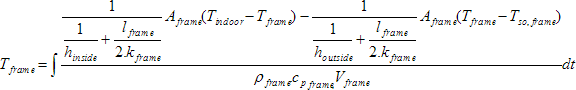 (13)
[K]
(13)
[K]
Energy balance equation of roof can be expressed by the following equation [7]:
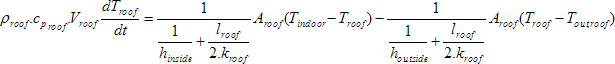 (14)
[W]
(14)
[W]
Where
- ρroof
- is density of concrete layer of roof [kg/m3]
- croof
- – specific heat capacity of concrete layer of roof [J/kg.K]
- Vroof
- – volume of concrete layer of roof [m3]
- Tout, roof
- – temperature out roof [K], where, space above the roof is not externally, but there is a mechanical equipment room which is located directly above the roof. Its temperature has been obtained by direct measurement.
By rearranging equation (14), Troof can be calculated as follows:
 (15)
[K]
(15)
[K]
The window glass transmits part of the incident solar radiation into the indoor space. While the solar radiation penetrates the glass pane, some of the energy will be absorbed by the glass, leading to an increase in the glass temperature, which will cause heat to flow in both the indoor and the outdoor directions, first by conduction within the glass and then by convection and radiation at the surfaces at both sides.
Heat Transferred through the window can be expressed by the following equation [9]:
Where
- Qwindows
- is heat exchange through windows [W]
- Awnidows
- – windows area [m2]
- Uwindows
- – overall heat transfer coefficient of windows [W/m2.K]
- Tso,windows
- – sol-air temperature for windows [K]
- Tindoors
- – temperature indoor [K]
- I
- – solar radiation incident on the window [W/m2]
- SC
- – solar heat gain coefficient

Fig. 6 SIMULINK model
After connecting all the sub-models, according to the balance of energy expressed in the previous equations, SIMULINK model will be obtained, as shown in Figure 6.
4. Results
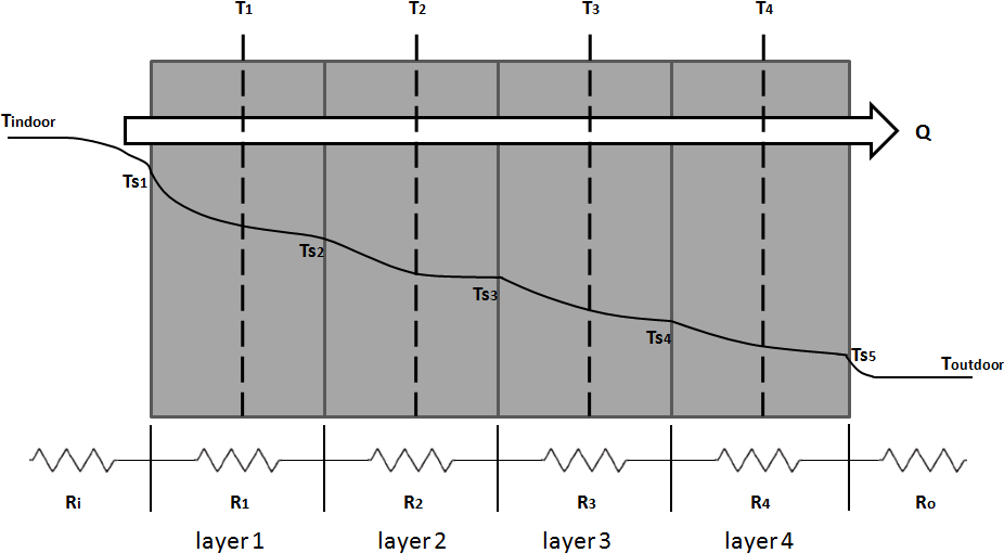
Fig. 7 Wall layers and their thermal network
To run simulation, the initial temperatures of all layers must be calculated based on the following methodology as computational boundary conditions. as shown in Figure 7.
Where, each element of the total thermal resistance through the wall can be calculated as follows:
Where
- R1, R2, R3, R4
- are thermal resistances of layers: wood, concrete, brick, concrete, respectively [m2.K/W]
- Ri, Ro
- – thermal resistances of inside and outside surfaces, respectively [m2.K/W]
By knowing (Tindoor) at time 00:00 from EBI system, and (Toutdoor) from TUBO data, temperature of all layers can be calculated for steady-state as follows:
After converting TUBO data into MAT files by using MATLAB/SIMULINK, it is possible to plot data in charts as shown in Figure 8. Where, simulation is applied on 8th August in 2013.
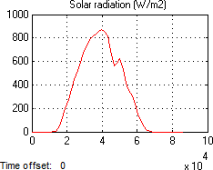
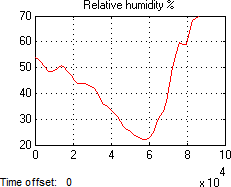 Fig. 8 Meteorological data outdoors recorded by TUBO station
Simulation period is from 7:30 till 15:00. There was no occupancy during this period. The results are shown in Figure 9.
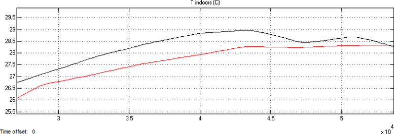
Fig. 9 Results (modelling and measurements, black: simulation result, red: values monitored by Honeywell system
Through the comparison between the simulation results and measurements showing that there is symmetry to a large extent between the results. Sometimes there are differences, are caused by factors have been neglected in the modelling process, such as calculation of air leakage, or some other climatic factors have not been taken into account.
What distinguishes the results is that the dynamic behaviour of the indoor temperature in the model largely simulates the dynamic behaviour of the real temperature. Meaning that the effect of solar radiation in the simulation has a similar role to the real impact. What gives an indication that the values provided by the TRNSYS model about the intensity of solar radiation on the external surfaces, and which are used later in the energy balance equations in SIMULINK model are close to a large extent from the real values, as well as the methodology used to solve the differential equations for the heat balance through the building envelope
5. Conclusion
The basic physical processes within classrooms have been modelled using MATLAB/SIMULINK software. In order to accomplish this task, the outdoor boundary conditions had to be specified with the used of weather data obtained from the meteorological station in Brno (TUBO).
With regard to the values of the intensity of solar radiation, a sub-model has been designed by using TRNSYS software to calculate the intensity of solar radiation incident on the walls of the building, with the help of the values of temperature, relative humidity and the intensity of solar radiation taken from the meteorological station.
Modelling the indoor temperature is based on the principle of conservation of energy. The main flows of energy to and from the building through the envelope have been modelled.
Convergence between simulation results and measurements paves the way for the development of the model to include sub-models for HVAC systems which can be designed based on the results of modelling of indoor environment presented in this work.
References
- [1] WANG, S. K. and Z. LAVAN. Air-Conditioning and Refrigeration. Mechanical Engineering Handbook Ed. Frank Kreith Boca Raton: CRC Press LLC, 1999.
- [2] De WIT, M. H. and H. H. DRIESSEN. ELAN A Computer Model for Building Energy Design. Building and Environment, 1988, 23(4), 285–289.
- [3] TUBO. Technical University BrnO, (Permanent GPS stations), 1994 [viewed 10 June 2012]. Available from: http://tubo.fce.vutbr.cz/new/
- [4] AL-RAWAHI, N. Z, Y. H. ZURIGAT and N. A. AL-AZRI. Prediction of Hourly Solar Radiation on Horizontal and Inclined Surfaces for Muscat/Oman. The Journal of Engineering Research, 2011, 8(2), 19–31.
- [5] KLEIN, S. A., et al. TRNSYS 16 – A Transient System Simulation Program. University of Wisconsin-Madison Solar Energy Laboratory, Madison, WI, USA. 2007.
- [6] SASIC KALAGASIDIS, A. The whole model validation for HAM-Tools. Case study: hygro-thermal conditions in the cold attic under different ventilation regimes and different insulating materials. Report R:03-6. Department of Building Technology, Chalmers University of Technology, Gothenburg, Sweden. 2003.
- [7] SOLEIMANI-MOHSENI, Mohsen. Modelling and intelligent climate control of buildings. Ph.D. thesis, Chalmers University of Technology, 2005.
- [8] JAMIL AHMAD, M., G. N. TIWARI, Singh ANIL KUMAR, Sharma MANISHA and H. N. SINGH. Heating/Cooling Potential and Carbon Credit Earned for Dome Shaped House. International Journal of Energy and Environment. 2010, 1(1), 133–148. ISSN 2076-2895.
- [9] ZHONG, Zhipeng and James E. BRAUN. Combined heat and moisture transport modelling for residential buildings. Indiana, Purdue University. 2008.
Článek se zabývá návrhem a posouzením počítačového modelu pro výpočet teploty vzduchu v interiéru místnosti během letního dne při aktivní tepelné zátěži od slunečního záření. Model zahrnuje tepelnou bilanci hlavních tepelných toků formujících výslednou teplotu vzduchu – tepelné zisky prostupem neprůsvitnými obvodovými konstrukcemi se zohledněním tepelné kapacity vrstev konstrukce a sáláním prosklenými konstrukcemi. Výpočet využívá vstupní data okolních podmínek budovy měřená místní meteorologickou stanicí, která přepočítává model v programu TRNSYS pro hlavní výpočet, který zajišťuje model v prostředí MATLAB – SIMULINK. Článek zahrnuje detailní popis modelu a prezentuje výsledky pro letní den. V závěru článku je prokázána dobrá shoda vypočtených dat s měřenými měřicím systémem budovy.
The actual indoor temperature is represented by a complex interaction between losses and gains, which contribute through a large number of variables on the energy balance. These variables are continuously changing, because the temperature outdoors is changing with time, as well as the solar heat gains and the internal heat gains.
In this work, a computer model has been designed by using TRNSYS software and MATLAB/SIMULINK software to simulate indoor temperature in summer. The building considered in this work is a lecture room at the Faculty of Mechanical Engineering at the Brno University of Technology. Where, the model of solar radiation incident on the external walls has been designed using TRNSYS software by exporting the real data taken from meteorological station in Brno (TUBO station) to the model, so that the intensity of solar radiation on each wall can be calculated and became usable in the SIMULINK model in order to calculate indoor temperature.
To make sure of the validity of the results, they have been compared with those recorded by a monitoring system installed in the building. Results have shown a significant convergence between simulation and measurements.